In a previous post, I have provided a statistical confirmation of the effective market theory on the stocks V, AAPL, SBUX, and NFLX. However, understanding that a market might be effective, and that technical analysis on single stocks may not yield returns with positive expectations, doesn't mean the market ceases to be profitable. That's because the geometric Brownian has a positive expectation for long term returns despite that of its index being kept at 0. But at precisely what time-scales will the expectation grow to be positive? And how are these returns distributed at any given time $t$? Here I will try to provide a theoretical derivation on the expected returns of a portofolio of $m$ independent stocks.
Model Setup
We start with the premise that there are "sufficiently large" number of mutually independent stocks in our portofolio, each described by a zero drift geometric random walk of the same index volatility $\nu$ with unit $1/\sqrt{\text{day}}$. This way the expected return is reliably estimated by the expectation $\E$ of the geometric normal distributions. Then at time $t$, under the assumption of random walk, the variance of each stock index will be:
$$\sigma^2 = \nu^2 t.$$
The stock indices of our portofolio follow distribution $K\sim N(\nu^2t, 0)$ at time $t$. We can then estimate the expected return of the portofolio by:
\begin{align}
\E\{e^K\} &= \frac{1}{\sqrt{2\pi\nu^2 t}}\int_{-\infty}^{\infty} e^{-\frac{k^2}{2\nu^2t}}e^kdk \tag{1}\\
&= \frac{1}{\sqrt{2\pi\nu^2 t}}\int_{-\infty}^{\infty} e^{-\frac{1}{2\nu^2t} (k^2-(2\nu^2t)k+(\nu^2t)^2)+\frac{(\nu^2t)^2}{2\nu^2 t}}dk \tag{2}\\
&=\frac{1}{\sqrt{2\pi\nu^2 t}}\int_{-\infty}^{\infty} e^{-\frac{(k-\nu^2t)^2}{2\nu^2t} }e^{\frac{\nu^2 t}{2}}dk \tag{3}\\
&=e^{\frac{\nu^2 t}{2}}\frac{1}{\sqrt{2\pi\nu^2 t}}\int_{-\infty}^{\infty} e^{-\frac{(k-\nu^2t)^2}{2\nu^2t} }dk \tag{4}\\
&=e^{\frac{\nu^2 t}{2}} \tag{5}
\end{align}
We can verify the conclusion that $\E = e^{\frac{\nu^2 t}{2}}$ with monte carlo simulation. Set $\nu = 0.01/\sqrt{\text{day}}$, construct the random walk by taking a time step of $\delta t = 0.01$, at each time step, modify the price index by $\delta K\sim\sqrt{\delta t}C U(-\frac{1}{2},\frac{1}{2})$. To find the value of $C$, we need to calculate the standard deviation of each step $\delta K$ and make sure that it is equal to $\sqrt{\delta t} \nu$:
$$\text{std}(\delta K) = \sqrt{\delta t}\nu$$
$$\Rightarrow \text{Var}(\delta K) = \delta t \nu^2$$
$$\Rightarrow \frac{\delta tC^2}{12} = \delta t \nu^2$$
$$\Rightarrow C = \sqrt{12}\nu = 2\sqrt{3}\nu.$$
//code for generating the random walk:
public void simulateSqrt(double n, double volatility) {
	LinearizedData data = new LinearizedData();
	double y = 0;
	for(double x = 0; x<=10000; x+=n) {
		data.append(x, Math.exp(y));
		y+=(Math.random()-0.5)*Math.sqrt(n)*volatility*2*Math.sqrt(3);
	}
	datas.add(data);
}
From comparing the simulated average returns and our derived returns, we see that our derivation seems to reliably predict the long term expected return of the stock. Now what if we increase the volatility of the stocks? By our theory, we should expect the long term expected return increase. Keeping everything else the same and increasing volatility to $\nu = 0.05 /\sqrt{\text{day}}$:
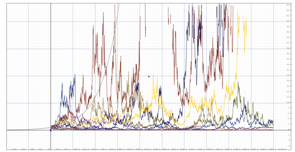
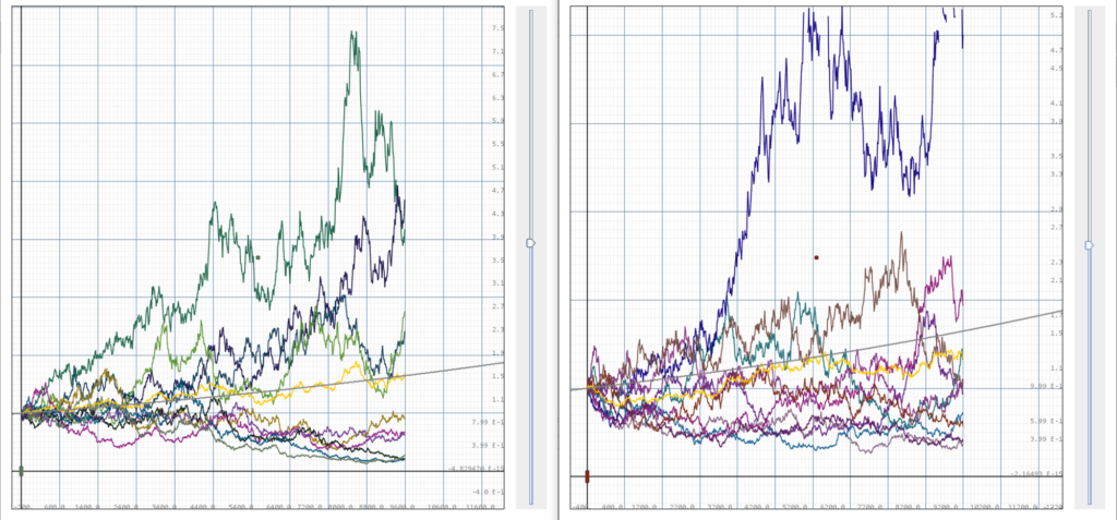
Here we can already see that the simulated return misses the theoretical return by large amounts, since the growth rate of the theoretical return is too large for linear scale visualization, we switch to log plots:
From the log plots comparisons, we can see that the simulated average return of high volatility portofolios often missed our theoretical expectance, and sometimes by large amounts (see plot 3, plot 1). This is because in calculating the expectation $\E$ of high volatility stocks, it is often difficult to have enough stocks to cover the range of returns $e^K$ where $K$ become extremely large, when we only have a portofolio of finite independent stocks. This requires us to go back to our premise and modify the "sufficiently large" assumption, as our stock portofolio is in fact finite, and the return distribution necessarily have something to do with the number of stocks we are simultaneously holding.
Finite Stock Portofolio
If we started with a portofolio of $m$ stocks, each following return distribution $R_i = e^{K_i}$ where $K\sim N(\nu \sqrt t, 0)$, and each are independent from each other, the net return distribution is that of $\sum_{i=1}^m R_i$. Computing the distribution of this sum directly will be difficult, as it involves convolution of distributions that are not analytically solved. Alternatively, we set a threshold $P_t$ for our return profile, and disgard all values of $e^K>P_t$ when calculating the expectation, as stocks with prices larger than $P_t$ at $t$ have "small probability" of being reached. Formally, we compute the conditional expectation that all stocks have values less than $P_t$ at time $t$.
Then we can take directly from (4) and obtain (with $C=\mathbb P \{R_i\leq P_t\}$):
\begin{align}
\E\{e^K|K\leq \ln(P_t)\} &=e^{\frac{\nu^2 t}{2}}\frac{1}{\sqrt{2\pi\nu^2 t}}\int_{-\infty}^{\ln(P_t)} e^{-\frac{(k-\nu^2t)^2}{2\nu^2t} }dk/C \tag{5}\\
&=e^{\frac{\nu^2 t}{2}} \frac{1}{\sqrt{2\pi\nu^2 t}}\int_{-\infty}^{\ln(P_t)} e^{-\frac{(k-\nu^2t)^2}{2\nu^2t} }d(k-\nu^2 t)/C \tag{6}\\
&=e^{\frac{\nu^2 t}{2}} \frac{1}{\sqrt{2\pi}}\int_{-\infty}^{\ln(P_t)} e^{-\frac{((k-\nu^2t)/\nu\sqrt{t})^2}{2} }d\frac{k-\nu^2 t}{\nu\sqrt t}/C \tag{7}\\
&=e^{\frac{\nu^2 t}{2}}\frac{\frac{1}{2}+\frac{1}{2}\text{erf}\left(\frac{\ln (P_t) -\nu^2t}{\sqrt{2t}\nu}\right)}{C} \tag{8}
\end{align}
Equivalently, we let $n$ be the number of standard deviations away from 0 that $\log(P_t)$ is set to be at time $t$. Then $P_t = e^{\sigma n} = e^{\nu \sqrt{t} n}$ and for each individual stock at time $t$, $$\mathbb{P}\{R_i \leq P_t\} = \frac{1}{\sqrt{\mathbb{2\pi}}} \int_{-\infty}^n e^{-\frac{t^2}{2}}dt = \frac{1}{2} +\frac{1}{2}\text{erf}\left(\frac{n}{\sqrt{2}}\right). \tag{9} $$
Then we get
\begin{align}
\E\{e^K|K\leq \ln(P_t)\} &=\frac{\frac{1}{2}+\frac{1}{2}\text{erf}\left(\frac{\ln (P_t) -\nu^2t}{\sqrt{2t}\nu}\right)}{\mathbb{P}\{e^K \leq P_t\}} \tag{10}\\
&=e^{\frac{\nu^2 t}{2}}\frac{\frac{1}{2}+\frac{1}{2}\text{erf}\left(\frac{\nu \sqrt{t} n-\nu^2t}{\sqrt{2t}\nu}\right)}{ \frac{1}{2} +\frac{1}{2}\text{erf}\left(\frac{n}{\sqrt{2}}\right)} \tag{11}\\
\E\{e^K|K\leq \ln(P_t)\}&=e^{\frac{\nu^2 t}{2}}\frac{\Phi(n-\nu\sqrt{t})}{ \Phi(n)} \tag{12}
\end{align}
This fascillitates the selection of a threshold $n$ for estimation. For a valid cutoff, the $\mathbb P$ that no $\log(R_i) > n\sigma$ should be no larger than, let's say $\mathbb P = 10%$, for in that case the conclusion drawn have a high $\mathbb P$ to be vacuous, as there is a P chance that the prices above the cutoff are never reached.
Now for a portofolio of $m$ stocks, the probability that all its stocks have values less than $P_t$ at time $t$ is:
$$\mathbb P\{R_i \leq P_t, \forall i \in [m]\} = \mathbb P\{R_i \leq P_t\}^m =\Phi(n)^m \tag{13}$$,
then the probability that there is at least 1 stock with value larger than $P_t$ is:
$$\mathbb P\{R_i > P_t, \exists i \in [m]\} =1- \mathbb P\{R_i \leq P_t\}^m =1-\Phi(n)^m \tag{14}.$$
The combination of (14) and (12) gives a parameterization of the distribution of return of a portofolio of $m$ independent stocks each with a volatility of $\nu$ by:

This commutative diagram defines an auxilary function $F(E,t,m, \nu)$ that is implicitly given by inverting $\mathbb E(n, t, \nu)$ with respect to $n$. To interpret $F$, we may note that $\mathbb P$ is the probability that there is at least one stock exceeding the cutoff, and in that case the conditional expectation of the return of our portfolio would be greater or equal to that given by $\mathbb E(n,t,\nu)$, which is the expectation that no stocks exceeds the cutoff. This gives a good approximation to the cumulative probability that the average return of the portofolio $\frac{1}{n}\sum_{i=1}^m R_i$ exceeds the given expectance $\mathbb{E}$. Though there is a difference between the average return and our conditional expected return. In general, the conditional expectation will be slightly lower than the average return corresponding to the same probability, and hence still provides a valid lower bound for return.
We may also use invert this diagram to find the return "expectance" $E(P, t,m, \nu)$, that finds the expected return for a portofolio of $m$ stocks, at a time $t$, with a certainty of $P$.

In this relation, we can explicitly compute $n$ from P by:
$$n(P, m) = \Phi^{-1}((1-P)^{\frac{1}{m}}),$$
and find corresponding expectance to be:
$$E(P, t, m) = e^{\frac{\nu^2 t}{2}}\frac{\Phi(n(P,m)-\nu\sqrt{t})}{\Phi(n(P,m))}.$$
To interpret this expression, we again see it as an approximation to the lower bound of the portofolio average return. If we take $P=0.5$, then at any time $t$, we expect a 50% chance to see our portofolio return to be above $E$, and 50% chance to see our portofolio return to be below $E$. Additionally, the distribution of portofolio returns should be concentrated around $E$ following the probability density function:
$$f(R,t,m,\nu) = \frac{d}{dE} F(E, t, m \nu)\biggr|_{E=R}.$$
We can plot these functions, to see what they look like. Again, with volatility $\nu=0.05$ and $m=10$, we take $P\in{0, 0.25,0.5,0.75}$,
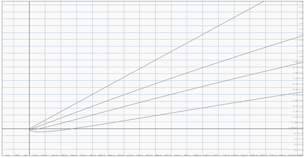
Mathematically, we can see that when $P=0$, $n=\infty$, $E=e^{\frac{\nu^2 t}{2}}\frac{\Phi(\infty-\nu\sqrt{t})}{\Phi(\infty)}=e^{\frac{\nu^2 t}{2}}\frac{1}{1}=e^{\frac{\nu^2 t}{2}},$ which reduces to our original expectation for infinite stock portofolio. Of course, as the conditional expectations only provide lower bounds for average return distributions, it is still possible for portofolio returns to exceed $E(P=0, t, m, \nu)$. But through Monte-Carolo simulations, we can see that the bound provided by $E(P, t, m, \nu)$ becomes tighter for higher volatilities $\nu$.
//Code for plotting expectance curves
static void plotExpectance(DataFrame2D frame) {
	for(double p = 0; p<=1-0.25; p+=1.0/4) {
		double n = ERF.IPhi(Math.pow(1-p, 1.0/m));
		Function1V correctedExpectance =
			new Function1V((t)->t[0]*volatility*volatility/2
		+Math.log(ERF.Phi(n-volatility*Math.sqrt(t[0]))/ERF.Phi(n)));
		correctedExpectance.setColor(Color.GRAY);
		frame.dataPane.addDataset(correctedExpectance);
	}
}
We shall perform Monte-Carlo on 10 portofolios, each of 10 independent stocks of volatilities 0.05, and observe their returns. For the expectance curve, we take $P=0.5$, and expect to see that at least half of the time, the portofolios outperform $E(P=0.5, t, m,\nu)$.
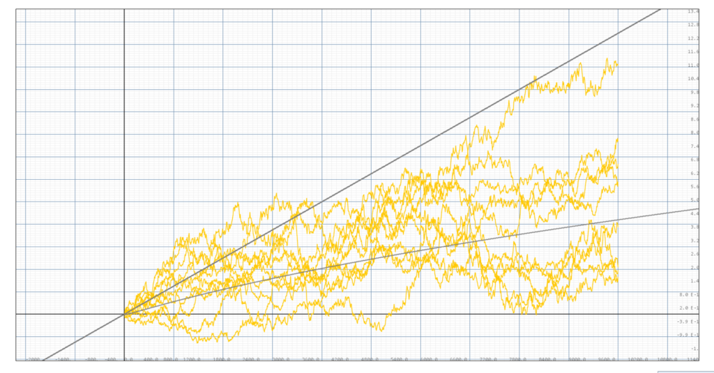
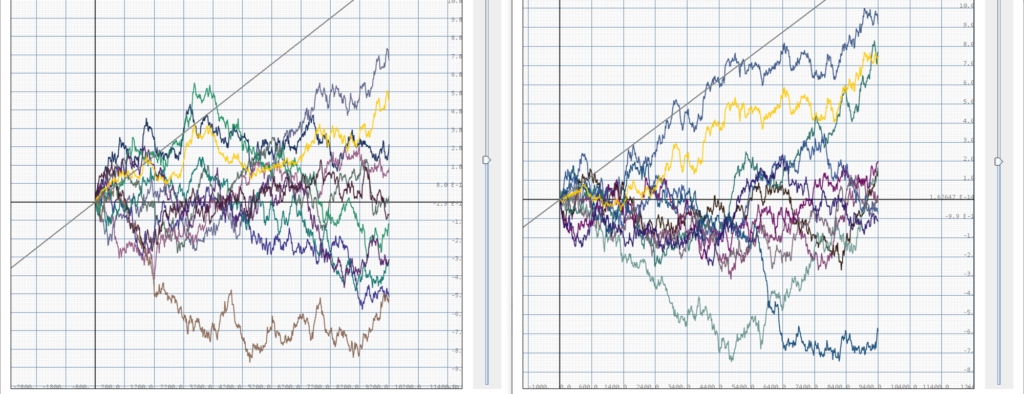
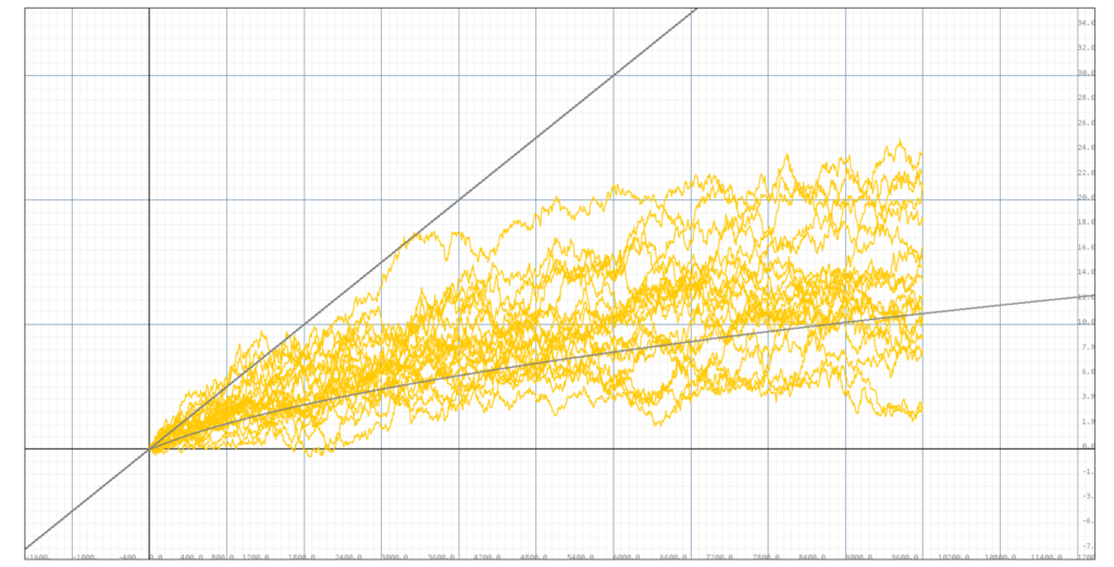
Simulation of 10 portofolios with volatility 0.05, portofolio size m=10, the light gray line below is the finite portofolio expectance for P=0.5. The dark gray line above is the growth expetation without the threshold.
We can see from the simulation above that our theoretical expectance does bounds approximately 50% of the stock returns from below. When the sample size increases, we can see that this bound is slightly vacuous. In the below simulation of 20 portofolios, we can see that 7 out of 20 returns were lower than the expectance, leaving slightly more than 50% above the expectance. It can thus be known that when the volatility is 0.05, the bound given is slightly vacuous.
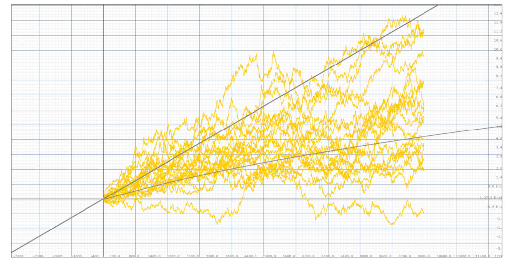
Simulation of 20 portofolios with volatility 0.05, portofolio size m=10, the light gray line below is the finite portofolio expectance for P=0.5. The dark gray line above is the growth expetation without the threshold.
Now let's increase the volatility to 0.1,
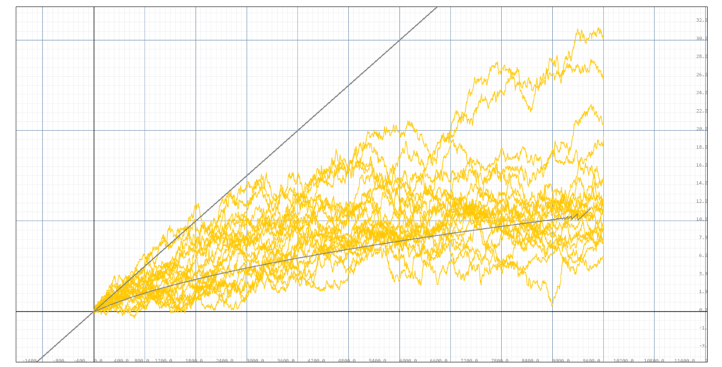
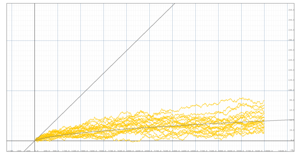
Simulation of 20 portofolios with volatility 0.1, portofolio size m=10, the light gray line below is the finite portofolio expectance for P=0.5. The dark gray line above is the growth expetation without the threshold.
it can be observed that the majority of all portofolios underperforms the return expectation without threshold, and that about half (8/20) of the portofolios underperform the P=0.5 expectance curve. There is also the issue of the discontinuity of the expectance curve for $t>8600$.
ERF.Phi(n-volatility*Math.sqrt(t[0]))
Function1V correctedExpectance =
			new Function1V((t)->t[0]*volatility*volatility/2
		+Math.log(ERF.Phi(n-volatility*Math.sqrt(t[0]))/ERF.Phi(n)));
In the above code snippet, we recognize that this is because ERF.Phi(n-volatility*Math.sqrt(t[0])) evaluates to 0 for n-volatility*Math.sqrt(t[0]) < -7, and hence Math.log(ERF.Phi(n-volatility*Math.sqrt(t[0])) evaluates to NaN. This is due to the limitation to the precision of Java double, but I devised this asymptotic extension to continue the evaluation of $\log(\Phi(x))$ for $x<-7$.
ERF.Phi(n-volatility*Math.sqrt(t[0]))
Function1V correctedExpectance =
			new Function1V((t)->t[0]*volatility*volatility/2
					+((n-volatility*Math.sqrt(t[0])>-7)?Math.log(ERF.Phi(n-volatility*Math.sqrt(t[0]))/ERF.Phi(n))
							:(-Math.log(volatility*Math.sqrt(t[0])-n)-Math.pow((volatility*Math.sqrt(t[0])-n), 2)/2-Math.log(ERF.Phi(n)))-Math.log(Math.sqrt(2*Math.PI)))
					));
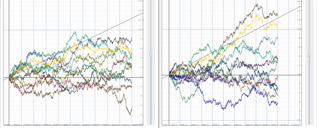
Simulation of 20 portofolios with volatility 0.1, portofolio size m=10, the light gray line below is the conditional expectance for P=0.5. The dark gray line above is the return expetation without the threshold.
Again, in this simulation, 8 out 20 portofolios under perform the conditional expectance, which is approximately half. But we can also see that more of the portofolio returns are clustered toward the conditional expectance compared to $\nu = 0.05$.
Now let's set the volatility to 0.3, and perform the simulations:
Simulation of 20 portofolios with volatility 0.3, portofolio size m=10, the light gray line below is the conditional expectance for P=0.5. The dark gray line above is the return expetation without the threshold.
We can see that this time, there are 10 portofolios, hence exactly 50% that underperformes our conditional expectance with $P=0.5$. Further, the returns are clustered closely around the conditional expectance curve rather than the full expectation curve, which significantly overestimates the return for highly volatile portofolios.
Portofolio Construction
Now that we have completed our theories on geometric brownian motions, we shall move on to constructing an actual portofolio in real world and find its expectance curve. From what we learned previously, it is for the best that we find stocks that are more volatile. But there is a catch --- the fluctuation in stock prices of individual stocks are not always independent from each other, so they cannot be considered as truly indendent geometric Brownian motions as we have considered in the above models. In that case, 10 correlated stocks cannot actually be considered as 10 independent stocks as did our previous model, but as some number less than that. Thus blindly putting more volatile stocks into a portofolio would not necessarily increase the return expectance (and would not necessarily be called "diversification").
In reality, the company stock prices are more or less correlated to the market, and it is difficult to find ones with negative correlations. So the best we can do is constructing a portofolio that have independent components beyond their common component of market.