After the large amount of backtesting of market neutral trading strategies that attempts to extract information from the historical price of a single stock to predict future prices, it was recognized that the portofolio returns often looked like random walks (no drift) without an overt effort for parameter tuning. It is thus worth asking, if there is any significant information extractable from the historical price of a stock without considering the market dynamic as a whole. Thus in this research, I attempt to verify the effective market hypothesis, and consider the possibility of profiting purely from market random walks.
Zeroth-order correlations
We start with a bucket of stock with historical data of accuracy up to minutes taken over the last three years. The bucket contains symbols V (dark blue), AAPL (light gray), SBUX (green), NFLX (red). We first take their historical indices to their e-based indices. Then we plot the indices at time $t$ as the $x$-coordinate and the indices at time $t+1$hr as the $y$-coordinate over the past 3 years. What we can see is a clear positive linear correlation, which tells that stock prices display temporal locality, in that percent changes to prices are small within an hour.
Code:
package test;

import java.awt.Color;
import java.io.IOException;
import java.util.ArrayList;

import codeLibrary.CSV;
import database.Datasheet;
import database.Function;
import database.LinearizedData;
import database.NoTimeEntryException;
import stockAnalyser.CalendarHelper;
import stockAnalyser.StockDatabase;
import ui.DataFrame2D;
import utils.Function1V;
import utils.Particles;
import stockCollector.Database;


public class LimitingPropagation {
	ArrayList<Function> datas = new ArrayList<Function>();
	ArrayList<LinearizedData> gains = new ArrayList<LinearizedData>();
	ArrayList<LinearizedData> rawInvestment = new ArrayList<LinearizedData>();
	ArrayList<LinearizedData> cashHolding = new ArrayList<LinearizedData>();
	double currentTime = CalendarHelper.getCurrentTimeStamp();
	static String[] symbols = new String[]  {"V", "AAPL", "SBUX", "NFLX"};
	public static void main(String[] args) {
		LimitingPropagation prop = new LimitingPropagation();
		for(int i = 0; i<symbols.length; i++) {
			prop.getHistoricPrice(symbols[i]);
			prop.simulateNetworthTrade(0.01, prop.datas.get(i));
		}
		prop.graph();
	}
	public void getHistoricPrice(String symbol) {
		Database database = Database.getDatabase(symbol);
		Datasheet datasheet = null;
		try {
			datasheet = database.assembleSheets();
		} catch (IOException e) {
			e.printStackTrace();
		} catch (NoTimeEntryException e) {
			e.printStackTrace();
		}
		LinearizedData price = datasheet.getColumn("price");
		double last = price.getLast().key;
		double org = price.get((5*0.0-3*24*365)*3600*1000+last);
		Function func = (t)->price.get((t-3*24*73)*3600*5000+last)/org;
		datas.add(func);
	}
	public void graph() {
		DataFrame2D frame = new DataFrame2D("");
		frame.setVisible(true);
		for(int i = 0; i<datas.size(); i++) {
			Function data = datas.get(i);
			Function1V function = new Function1V((t)->data.get(t[0]));
			Color color = new Color(StockDatabase.colors.get(symbols[i]));
			function.setColor(color);
			frame.dataPane.addDataset(function);

			Particles correlation = new Particles();
			double prevPrice = 1;
			for(double t = 1; t<1500; t+=1) {
				double currentPrice = data.get(t);
				correlation.addParticles(new double[] {Math.log(prevPrice), Math.log(currentPrice)});
				prevPrice = currentPrice;
			}
			correlation.setColor(color);
			frame.dataPane.addDataset(correlation);
		}
	}
}
First-order correlations
Next we measure the correlation for the percent changes in prices for a bucket. Namely, we are asking if the prices have gone up in the previous hour, are we expecting to see the prices to correspondingly go in the same direction or the opposite direction in this coming hour? If there is any correlation at all, there will always be a strategy that allows us to predict the stock price changes and make a profit. As for holding $h$, the changes in prices as $\delta p$, the differential profit $\delta w$ can be described by:
$$\delta w = h \delta p.$$
We plot the change in stock indices over the past hour as the $x$-axis and the change in this hour as the $y$-axis.
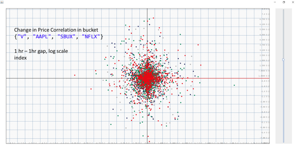
It is quite clear that the distribution of these points follow a largely symmetric radial pattern, showing the correlation to be 0. Hence showing it to be impossible to predict future price changes based on the stock indices change in the past hour. It is also clear that $\mathbb{E}\{\log(p(t+1))-\log(p(t))|\log(p(t))-\log(p(t-1))\}=0$
Code:
package test;

import java.awt.Color;
import java.io.IOException;
import java.util.ArrayList;

import codeLibrary.CSV;
import database.Datasheet;
import database.Function;
import database.LinearizedData;
import database.NoTimeEntryException;
import stockAnalyser.CalendarHelper;
import stockAnalyser.StockDatabase;
import ui.DataFrame2D;
import utils.Function1V;
import utils.Particles;
import stockCollector.Database;


public class LimitingPropagation {
	ArrayList<Function> datas = new ArrayList<Function>();
	ArrayList<LinearizedData> gains = new ArrayList<LinearizedData>();
	ArrayList<LinearizedData> rawInvestment = new ArrayList<LinearizedData>();
	ArrayList<LinearizedData> cashHolding = new ArrayList<LinearizedData>();
	double currentTime = CalendarHelper.getCurrentTimeStamp();
	static String[] symbols = new String[]  {"V", "AAPL", "SBUX", "NFLX"};
	public static void main(String[] args) {
		LimitingPropagation prop = new LimitingPropagation();
		for(int i = 0; i<symbols.length; i++) {
			prop.getHistoricPrice(symbols[i]);
			prop.simulateNetworthTrade(0.01, prop.datas.get(i));
		}
		prop.graph();
	}
	public void getHistoricPrice(String symbol) {
		Database database = Database.getDatabase(symbol);
		Datasheet datasheet = null;
		try {
			datasheet = database.assembleSheets();
		} catch (IOException e) {
			e.printStackTrace();
		} catch (NoTimeEntryException e) {
			e.printStackTrace();
		}
		LinearizedData price = datasheet.getColumn("price");
		double last = price.getLast().key;
		double org = price.get((5*0.0-3*24*365)*3600*1000+last);
		Function func = (t)->price.get((t-3*24*73)*3600*5000+last)/org;
		datas.add(func);
	}
	public void graph() {
		DataFrame2D frame = new DataFrame2D("");
		frame.setVisible(true);
		for(int i = 0; i<datas.size(); i++) {
			Function data = datas.get(i);
			Function1V function = new Function1V((t)->data.get(t[0]));
			Color color = new Color(StockDatabase.colors.get(symbols[i]));
			function.setColor(color);
			frame.dataPane.addDataset(function);

			Particles correlation = new Particles();
			double prevChange = Math.log(data.get(0.0)/data.get(-1.0));
			for(double t = 1.0; t<1500; t+=1) {
				double currentChange= Math.log(data.get(t)/data.get(t-1.0));
				correlation.addParticles(new double[] {prevChange,currentChange});
				prevChange = currentChange;
			}
			correlation.setColor(color);
			frame.dataPane.addDataset(correlation);
		}
	}
}
But what if we lengthen the time horizon of sampling? If the stock price has rised over the past 10 days, should we expect the stock prices to keep rising over the next hour? Conversely if the stock price droped over the past 10 days, should we expect the stock prices to keep droping over the next hour? We plot the change in stock indices over the past 10 days as the $x$-axis and the change in the next hour as the $y$-axis.
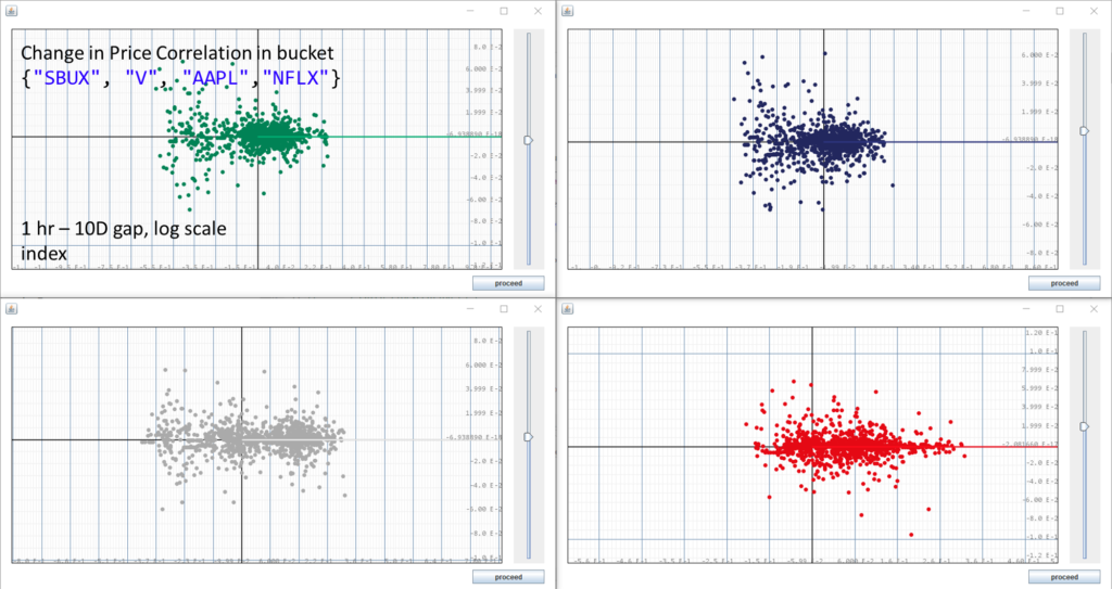
Here we see a larger variance in the $x$ direction (compared to the $y$ direction), as the price variations can be reasonably expected to be larger over the longer period of 10 days. But there still seems to be no significant correlation, as the data are symmetric across the $x$-axis, showing a covariance of roughly 0. There are some other patterns that we might detect, such as the more spread out hourly price change in the negative-$x$ quadrant, but as they are spread out symmetrically across the $x$-axis, we cannot make reliable predictions as the conditional expection stays at 0.
Second-order correlations
One may further wonder if there are second order correlations, which we may utilize to create profitable strategies. We plot the change in the stock price index change over the past hour given by $(\log(p(t))-\log(p(t-1)))-(\log(p(t-1))-\log(p(t-2)))$ compared to that over the current hour $(\log(p(t+1))-\log(p(t)))-(\log(p(t))-\log(p(t-1)))$.
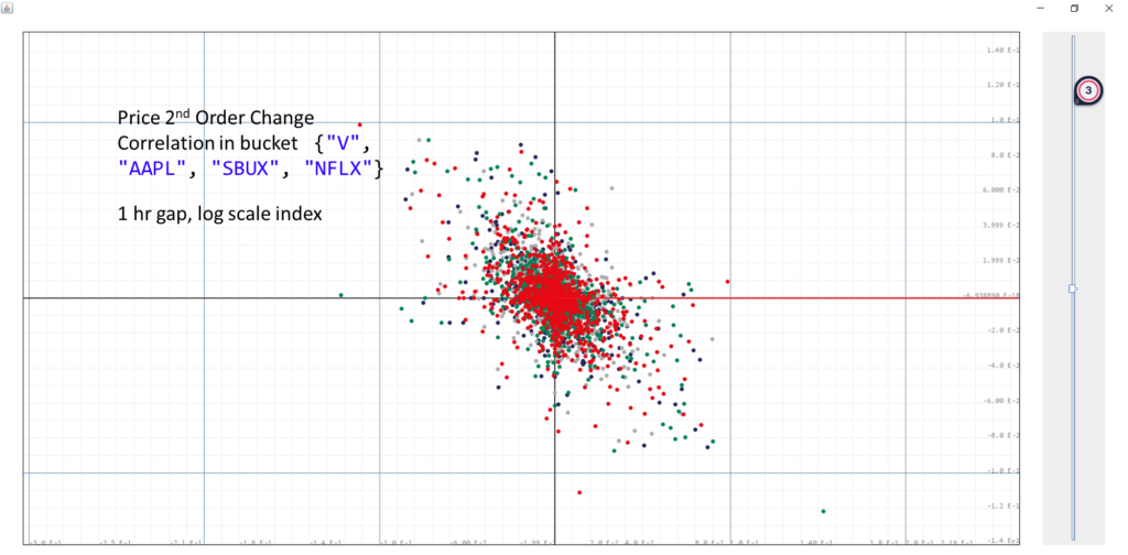
Here we see a clear negative correlation, meaning that the second order change in the previous hour is inversely correlated with that of this hour. But does that mean we have found a reliable way to extract information for stock price prediction? We shall compare these results to that of a actual random walk.
Updated Code in graph():
Particles correlation = new Particles();
double prevChange =(Math.log(data.get(0.0))-Math.log(data.get(-1.0)))
-(Math.log(data.get(-1.0))-Math.log(data.get(-2.0)));
for(double t = 1.0; t<1500; t+=1) {
double currentPrice = (Math.log(data.get(t))-Math.log(data.get(t-1.0)))
-(Math.log(data.get(t-1.0))-Math.log(data.get(t-2.0)));
correlation.addParticles(new double[] {prevChange,currentPrice});
prevChange = currentPrice;
}
correlation.setColor(color);
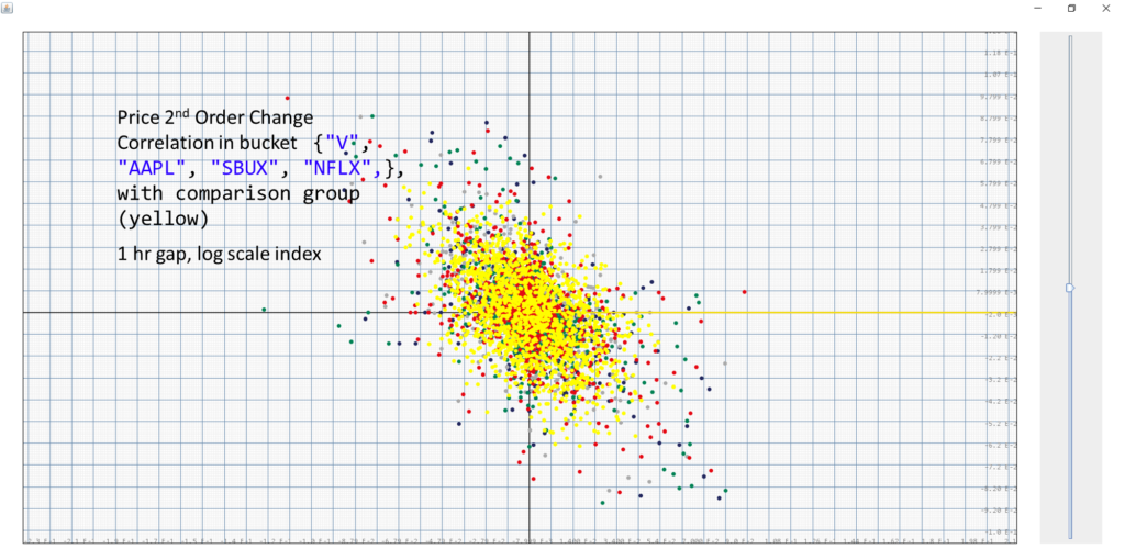
frame.dataPane.addDataset(correlation);We generate a comparison group using a neutral random walk with a similar volatility as our bucket average. As it turns out, the second order change of a random walk also had a negative correlation. Thus it is still impossible to make any predictions on the market based on second order changes.
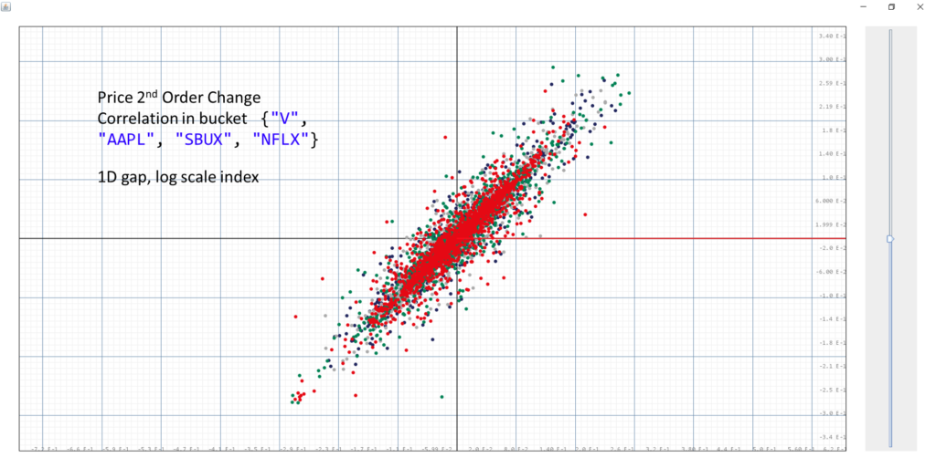
As we increase the measurement gap of the 2nd order change to 1 day while keeping the correlation time difference to be at an hour, we start to see a positive correlation. But this is easily explained by temporal locality and hence yield no valuable predictability.
We shall continue to compare this result with the random walk group:
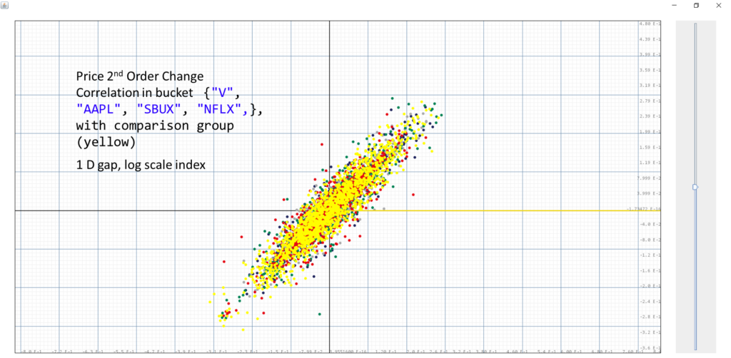
which as expected, still displayes strong agreement.
Conclusion
Stock markets locally follow in general a random walk pattern, this is seen in the comparison between the 1st , 2nd, 3rd order change measured locally, which means that it will be difficult to beat the market using local technical analysis.
On the other hand, disregarding drift, stock market locally follow geometric Brownian motions, that means the expectations of a bucket of stocks is always growing, we can compute this value by:
$$\int e^k e^{-\frac{k^2}{2σ^2 t}} dk=e^{-\frac{σ^2 t}{2}}.$$