Explaining Moving Average Noise Reduction With Fourier Transform

In stock analysis and other time sequenced data analysis, a lot of mathematical tools rely on a certain level of smoothness of the input data sequence. Moving average is often utilized to achieve this purpose, but moving averge also causes latency in information. So what is the optimal period for data smoothing using moving average to achieve the most noise reduction with the least information lost? I would like to use fourier transform to create a analytical approach for determing and explaining moving average.

Let $f$ be defined by $f:(\infty,x_0]\rightarrow \R $, where $x_0\in\R$. Assume that function $f$ is transformed in the form

$$f(x) = \sum_{i=1}^\infty a_i\cos(ix)+\sum_{i=1}^\infty b_i\sin(ix).$$

We define moving average operator $\bar{f}^{t}$ over a range $t\in\R$ as:

$$\ag{f}{t}(x)\equiv \frac{1}{t}\int_{x-t}^x f(x)dx.$$

Then by sum to product formula:

$$\begin{align*}
\ag{f}{t}(x)& = \frac{1}{t}\int_{x-t}^{x}\left(\sum_{i=0}^\infty a_i\cos(ix)+\sum_{i=1}^\infty b_i\sin(ix)\right)dx\\
&=a_0+\frac{1}{t}\sum_{i=1}^n\left[\frac{a_i}{i}(\sin(ix)-\sin(i(x-t))-\frac{b_i}{i}(\cos(ix)-\cos(i(x-t))\right]\\
&= a_0+\frac{1}{t}\sum_{i=1}^n\left[\frac{a_i}{i}2\cos\left(\frac{2ix-it}{2}\right)\sin\left(\frac{it}{2}\right)+\frac{b_i}{i}2\sin\left(\frac{2ix-it}{2}\right)\sin\left(\frac{it}{2}\right)\right]\\
&=\sum_{i=0}^\infty\frac{2\sin(\frac{it}{2})}{it}\left(a_i \cos\left(ix-\frac{it}{2}\right) +b_i\sin\left(ix-\frac{it}{2}\right)\right)
\end{align*}$$

For $i=0$ term in the summation above, we take the limit of $\frac{2\sin\left(\frac{it}{2}\right)}{it}=1$.

Letting $\phi = \frac{t}{2}$ which we may dub the name "phase shift", we have that:

$$\ag{f}{t}(x)=\sum_{i=0}^\infty \frac{2\sin\left(\frac{it}{2}\right)}{it} \left(a_i\cos(i(x-\phi))+b_i\sin(i(x-\phi))\right).$$

Rewriting this in the frequency domain, we can see that:

$$\begin{equation}
\left\{
\begin{aligned}
F_c(\omega,\ag{f}{t}(x))&=\frac{2\sin\left(\frac{\omega t}{t}\right)}{\omega t}F_c(\omega, f(x-\phi))\\
F_s(\omega,\ag{f}{t}(x))&=\frac{\sin\left(\frac{\omega t}{2}\right)}{\omega t}F_s(\omega,f(x-\phi)).
\end{aligned} \right.
\end{equation}$$

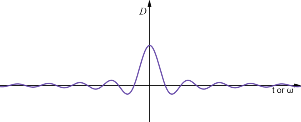
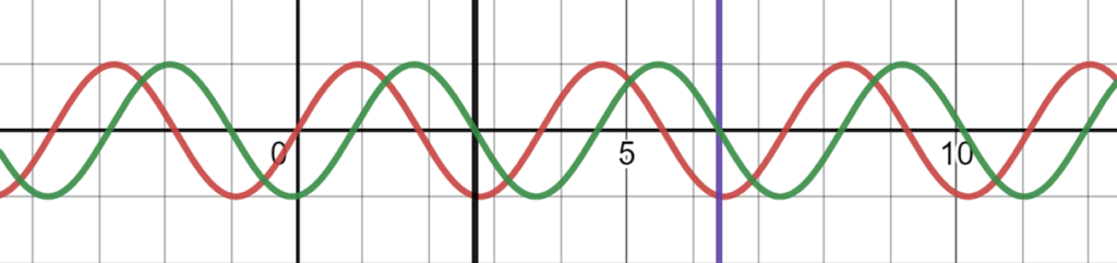
This result reveals two interesting things about moving average. First, we get to quantify the information latency caused by taking averages, that is, the smoothed function is delayed by a phase shift of $\phi=\frac{t}{2}$ compared to the original function. Second, we see that after the averaging, all amplitudes of the underlying harmonics are damped by $D(\omega t)=\frac{2}{\omega t}\sin\left(\frac{\omega t}{2}\right)\leq 1$.

For fixed $\omega$ or $t$, we have $D$ decaying w.r.t. $t$ or $\omega$:

Another rule that can be easily proven is that:

$$F(\omega, \ag{f'}{t}(x))=D(\omega t)F(\omega, f'(x)).$$

Since for $f(x) = \sum_{i=0}^\infty a_i\cos(ix)+\sum_{i=1}^\infty b_i\sin(ix)$, $$f'(x)=\sum_{i=0}-ia_i\sin(ix)+\sum_{i=1}^\infty b_i\cos(ix).$$

That is,
$$\begin{equation}
\left\{
\begin{aligned}
F_c(\omega,f'(x))&=-\omega F_s(\omega,f(x))\\
F_s(\omega,f'(x))&=\omega F_c(\omega,f(x)).
\end{aligned} \right.
\end{equation}$$
Thus,
$$\begin{equation}
\left\{
\begin{aligned}
F_c(\omega,\ag{f'}{t}(x))&=D(\omega t) F_c(\omega,f'(x))=\omega D(\omega t)F_s(\omega, f(x-\phi))\\
F_s(\omega,\ag{f'}{t}(x))&=D(\omega t) F_s(\omega,f'(x))=-\omega D(\omega t)F_c(\omega, f(x-\phi)).
\end{aligned} \right.
\end{equation}$$

Targetted Noise Reduction with Moving Average

Now we want to use this property of moving average, to study how to extract the noise frequency from arbitrary functions. We also want to know, given a noise frequency, how to eliminate it with the least amount of information loss (latency).

To find general form of fourier transform on any range $[a,b]$, we let $T = b-a$. Then the Hilbert space of $f:[a,b]\rightarrow \R$ is spaned by orthogonal basis $$\cos\left(n\frac{2\pi}{T}x\right), \sin\left(n\frac{2\pi}{T}x\right), n\in \N.$$

Let $c_n= \left<f,\cos\left(n\frac{2\pi}{T}x\right)\right>, s_n=\left<f,\sin\left(n\frac{2\pi}{T}x\right)\right>$, then

$$F_c\left(n, f(x)\right)\equiv c_n=\frac{\int_a^bf(x)\cos\left(n\frac{2\pi}{T}x\right)dx}{\int_a^b\cos^2\left(n\frac{2\pi}{T}x\right)dx}=\frac{2\int_a^bf(x)\cos\left(n\frac{2\pi}{T}x\right)dx}{b-a},$$
similarly
$$F_s\left(n, f(x)\right)\equiv s_n=\frac{2\int_a^b f(x)\sin\left(n\frac{2\pi}{T}x\right)dx}{b-a}.$$

Since damping factor of $F(\omega, \ag{f}{t}(x))$ is equal to $D(\omega t) = \frac{2}{\omega t}\sin\left(\frac{\omega t}{2}\right)$, it can be easily observed that the amplitudes on the frequency domain are damped to 0 when $\frac{\omega t}{2} = \pi m \Rightarrow \omega=\frac{2\pi m}{t}, m\in \N$, which eliminates the noise composition in that frequency.

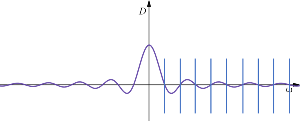
To minimize information loss, we take the lowest $t$ that satisfies $\frac{\omega_0 t}{2}=\pi \N$, for a function with noise frequency $\omega_0$. Consequently, the noise elimination period $t$ for a single noise frequency $\omega$ is $t=\frac{2\pi}{\omega_0}$. Since $\omega_0=\frac{2\pi n_0}{T}$, we can also compute $t$ directly from the principle noise index $n_0$: $$t=\frac{2\pi}{n_02\pi}T=\frac{T}{n_0}=\frac{b-a}{n_0}.$$

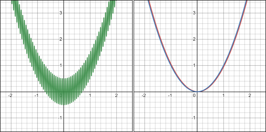
For instance, if we already know the function is $f(x)=x^2+0.5\sin(100x)$ is subject to a noise frequency of $\omega = 100$, then we shall eliminate it with $t=\frac{2\pi}{100}$. In terms of moving average, we have smoothed function: $$\ag{f}{\frac{2\pi}{100}}(x) = \frac{100}{2\pi}\int_{x}^{x+\frac{2\pi}{100}}\left(t^{2}+0.5\sin\left(100t\right)\right)dt=\left(x-\frac{\pi}{100}\right)^2.$$

We know that the smoothed function is phase shifted by $\phi = \frac{t}{2} = \frac{\pi}{100}$, so translating it to the left by taking $\ag{f}{\frac{2\pi}{100}}(x+\frac{\pi}{100})$ will restore the original function. Next, we will discuss how to extract the noise frequencies from a functions' Fourier spectrum.

Noise Reduction that avoids phase shift

As we see that taking average shifts all the component harmonics by $\phi = \frac{t}{2}$ before multiplying them by damping factors, a direct way to avoid this phase shift is by shfiting the averaging range by $\frac{t}{2}$, so that data taken at the point of averaging have the quality of symmetry. Thus we define mid-averaging $\hat{f}^t$:

$$\mg{f}{t}\equiv \frac{1}{t}\int_{x-\frac{t}{2}}^{x+\frac{t}{2}} f(x)dx,$$
such that $D(\omega t) = \frac{2}{\omega t} \sin(\omega t)$, and $\phi = 0$.

Finding the primary noise frequency

Observations about noise in time domain data:

1. Noise is relative. Noise from different frequencies might contribute useful informtion about the original function.
2. Noise is a high frequency harmonic component with abnormally high amplitude.
3. Taking average damps high frequency harmonic components and completely eliminates frequencies that are an integer multiple of it.

Based on these assumptions, we can try to discover the primary noise by looking at peaks on the frequency graph. As an experiment, we let $f:[a,b]\rightarrow \R, f(x)=1$, and we are expecting to see no peaks on the frequency domain:

$$\begin{align*}
F_c(n, f(x)=1) &= \frac{2}{b-a}\int_a^b 1 \cos\left(n\frac{2\pi}{b-a}x\right) dx \\
&= \frac{b-a}{2\pi n}\frac{2}{b-a}\left(\sin\left(\frac{2\pi}{b-a}nx\right)\Bigg|_a^b\right)\\
&= \frac{2}{\pi n } \cos\left(\frac{1}{2}\left(\frac{2\pi n (b+a)}{b-a}\right)\right)\sin\left(\pi n\right)\\
&= \frac{2}{\pi n} \cos\left(\pi n\left(\frac{b+a}{b-a}\right)\right)\sin(\pi n).
\end{align*}$$

As shown, the frequency graph isn't flat as expected. On the contrary, it has maximum at $n=0$, with value $F_n = 2$. This is explainable because the function $f(x)=1$ technically has a frequency It becomes 0 every time $n\in \Z \Rightarrow \sin(\pi n) = 0$, and diminshes over increasing $n$.

This phenomenum occurs with nearly all the functions $f$, and makes it difficult to find peaks on the frequency graph. Therefore, an approach is to find out the oscillation patterns in fourier transforms $F(n, f(x)$, and try to find ways to counter it.

Again, $$\begin{equation}
\left\{
\begin{aligned}
F_c\left(\omega =n\frac{2\pi}{T}, f(x)\right)&=\frac{\int_a^bf(x)\cos\left(n\frac{2\pi}{T}x\right)dx}{\int_a^b\cos^2\left(n\frac{2\pi}{T}x\right)dx}=\frac{2\int_a^bf(x)\cos\left(n\frac{2\pi}{T}x\right)dx}{b-a}\\
F_s\left(\omega =n\frac{2\pi}{T}, f(x)\right)&=\frac{\int_a^bf(x)\sin\left(n\frac{2\pi}{T}x\right)dx}{\int_a^b\sin^2\left(n\frac{2\pi}{T}x\right)dx}=\frac{2\int_a^b f(x)\sin\left(n\frac{2\pi}{T}x\right)dx}{b-a}.
\end{aligned} \right.
\end{equation}$$

For the $F_c$ term we have

$$\begin{align*}
\int_a^b &f(x) \cos \left(n \frac{2\pi}{b-a} x\right) dx\\
=&\frac{b-a}{2\pi n} \int_a^b d\sin\left(n\frac{2\pi}{b-a} x\right)\\
=& \frac{b-a}{2\pi n}\left[f(x) \sin \left(n\frac{2\pi}{b-a} x\right)\right] \Bigg|_a^b -\frac{b-a}{2\pi n}\int_a^b \sin\left(n\frac{2\pi}{b-a}x\right)f'(x)dx\\
=& \frac{b-a}{2\pi n}\left[f(x) \sin \left(n\frac{2\pi}{b-a} x\right)\right] \Bigg|_a^b -\left(\frac{b+a}{2\pi n}\right)^2\left[f'(x)\cos\left(n\frac{2\pi}{b-a}x\right)\right]^b_a\\
&-\left(\frac{b-a}{2\pi n}\right)^2\int_a^b\cos(n\frac{2\pi}{b-a} x)f''(x) dx\\
=& ...\\
=&\sum_{i=1}^\infty \left(\frac{b-a}{2\pi}\right)^i\frac{1}{n^i}\left[f^{(i-1)}(x) [\cos_{i \text{ even}}, \sin_{i \text{ odd}}]\left( n\frac{2\pi}{b-a} x\right) \right]^b_a(-1)^{\left\lfloor \frac{i}{2}\right\rfloor}
\end{align*}$$
Extracting factors of $n$, we get:

$$\int_a^b f(x)\sin\left(n \frac{2\pi}{b-a}x\right)dx = -\frac{c_1}{n}\cos(...)-\frac{c_2}{n^2}\sin(...)+\frac{c_3}{n^3}\cos(...)...$$

Since $\sin(x)\leq 1, \cos(x)\leq 1$, for functions that satisfy $[f^{(i)}(b)-f^{(i)}(a)]$ is a constant, it is gauranteed that further terms of the series diminishes to $0$ as $n$ increases.

One can hence obtain that asymptotically,
$$\begin{align*}
\lim_{n\rightarrow \infty} n F_c(n) &= \frac{2}{b-a}\frac{b-a}{2\pi}\left(f(x)\sin\left(n\frac{2\pi}{b-a}x\right)\right)^b_a= \frac{f(b)\sin\left(n\frac{2\pi}{b-a}b\right)-f(a)\sin\left(n\frac{2\pi}{b-a}a\right)}{\pi}\\
\lim_{n\rightarrow \infty} n F_s(n) &= \frac{2}{b-a}\frac{a-b}{2\pi}\left(f(x)\cos\left(n\frac{2\pi}{b-a}x\right)\right)^b_a= \frac{f(a)\cos\left(n\frac{2\pi}{b-a}a\right)-f(b)\cos\left(n\frac{2\pi}{b-a}b\right)}{\pi}
\end{align*}$$

From the asymptotic behaviors of $F_c(n)$ and $F_s(n)$, we can see that there is a leading residue of $\sin\left(n\frac{2\pi}{b-a}b\right)f(b)-\sin\left(n\frac{2\pi}{b-a}a\right)f(a)$ in the function. One can factor out these residues by taking $\hat{\cdot}^t$ on $nF_c(n)$ and $nF_s(n)$ s.t. $\exists k, l \in \Z$, $$\frac{\pi}{b-a}bt = k\pi, \frac{\pi}{b-a}at = l\pi.$$

A simpler way to resolve this disturbance is by shifting the orthogonal basis by $\phi = \frac{b+a}{2}$ in the first place, so that there will only be one oscillating disturbance on the frequency graph.

Then from, $$\begin{equation}
\left\{
\begin{aligned}
F_c\left(\omega =n\frac{2\pi}{T}, f(x)\right)&=\frac{2\int_a^bf(x)\cos\left(n\frac{2\pi}{T}\left(x-\frac{b+a}{2}\right)\right)dx}{b-a}\\
F_s\left(\omega =n\frac{2\pi}{T}, f(x)\right)&=\frac{2\int_a^b f(x)\sin\left(n\frac{2\pi}{T}\left(x-\frac{b+a}{2}\right)\right)dx}{b-a}.
\end{aligned} \right.
\end{equation}$$

from which we can deduce that:
$$\begin{align*}
\lim_{n\rightarrow \infty} nF_s(n) &= -\frac{1}{\pi}\left(f(x)\sin\left(\frac{2\pi n}{b-a}\left(x-\frac{b+a}{2}\right)\right)\right)^b_a\\
&=\frac{1}{\pi}\left(f(b)\sin\left(\frac{2\pi n}{b-a}\left(\frac{b-a}{2}\right)\right)-f(a)\sin\left(\frac{2\pi}{b-a}\left(\frac{a-b}{2}\right)\right)\right)\\
&= \frac{1}{\pi}(f(a)+f(b))\sin(\pi n)\\
\lim_{n\rightarrow \infty} nF_c(n) &= -\frac{1}{\pi}\left(f(x)\cos\left(\frac{2\pi n}{b-a}\left(x-\frac{b+a}{2}\right)\right)\right)^b_a\\
&=\frac{1}{\pi}(f(a)-f(b))\cos(\pi n)
\end{align*}$$
It becomes much simpler now, since there is only one residue frequency on $F_c$ and $F_s$ and its angular frequency is $\pi$, one can take the moving averaging of the function with $t$ s.t. $\frac{\omega t}{2} = \pi$, then $\frac{\pi t}{2} = \pi \Rightarrow t=2$. Avoiding the phase change, the noise frequency spectrum of $f(x)$ becomes:

$$P_c(n) = \widehat{nF_c}^2(n) = \int_{-1}^1 nF_c(n)dn, \ \ \ \ P_s(n) = \widehat{nF_s}^2(n) = \int_{-1}^1nF_s(n)dn.$$

We can then extract the noise frequencies by taking:
$$P(n) = P_c(n)^2+P_s(n)^2$$
where peaks on $P(n)$ correspond to major noise frequencies of the function. Then with these, frequencies, say $n_1, n_2, ...$, we can find the corresponding averaging periods following the formula $t=\frac{2\pi}{\omega} = \frac{b-a}{n}$.

Example for noise reduction

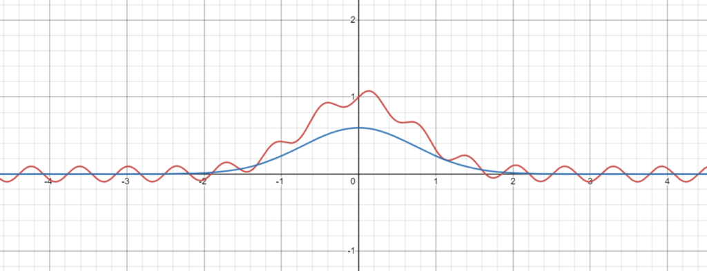
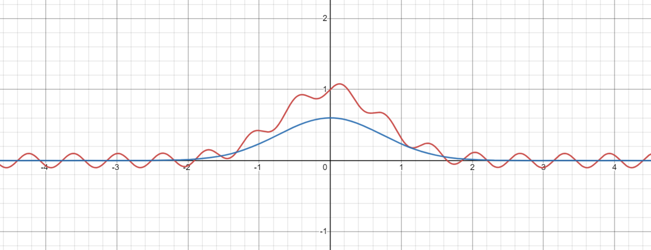
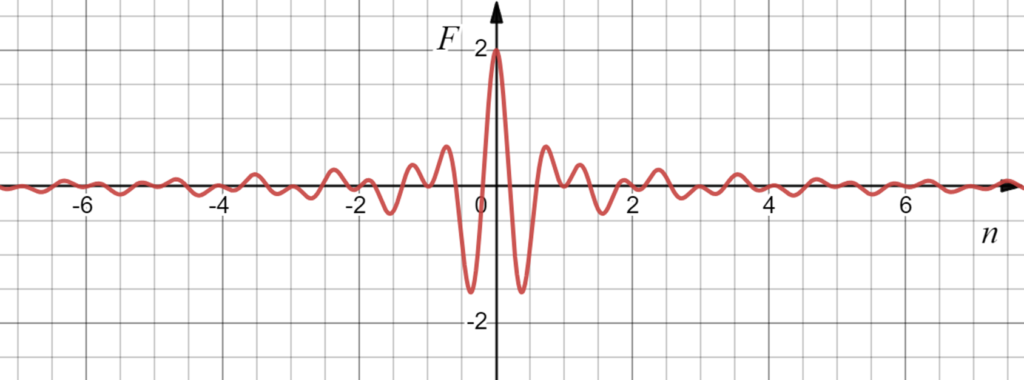
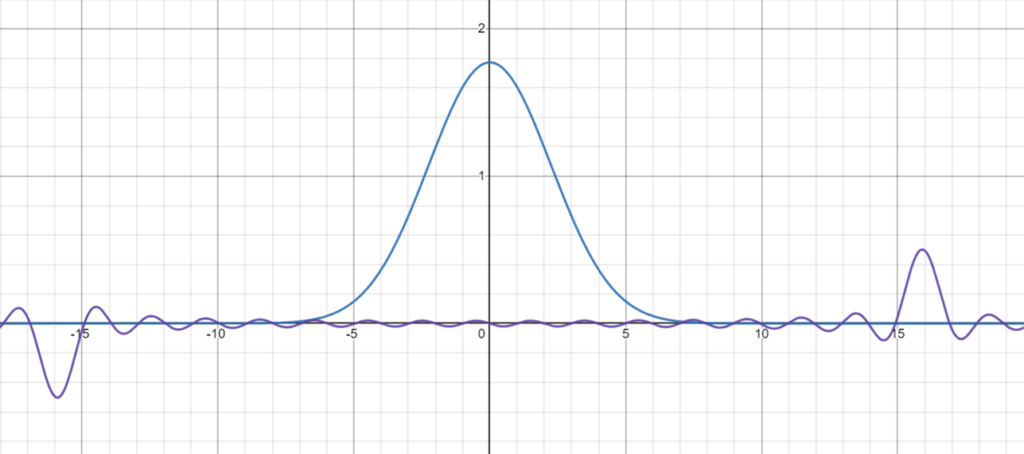
We can try to apply this technique numerically to example function $$f(x)=e^{-x^2}+\frac{\sin\left(10x\right)}{10}.$$ We take its DFT between domain $[-5,5]$.

Its fourier transforms:

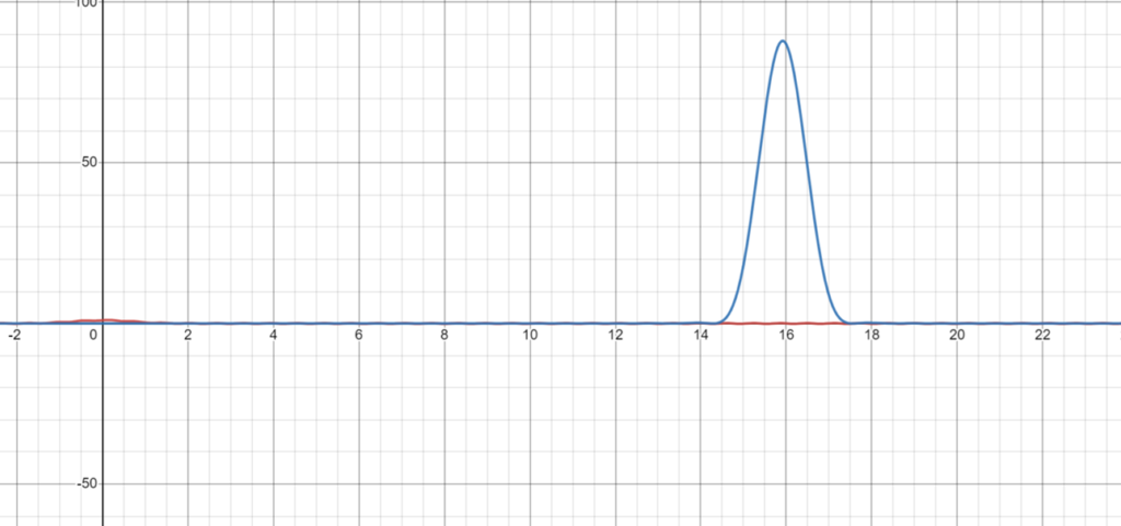
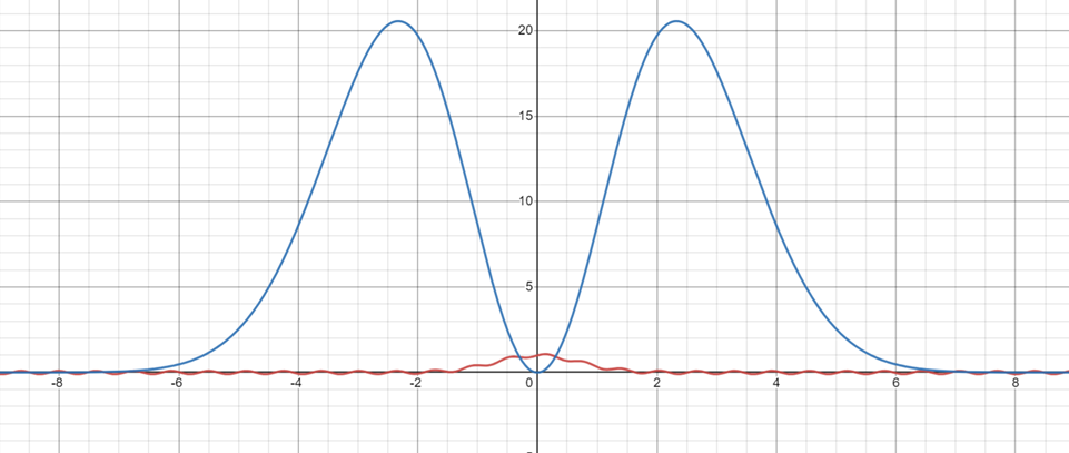
We can see then numerically compute $P_c(x)^2 = \left(\widehat{nF_c}^2\right)^2$ and $P_s(x)^2 = \left(\widehat{nF_s}^2\right)^2$

In general, we can numerically traverse the noise spectrum $P(n)$, and find the peak beyond a certain feature threshold $N_{f}$, to be considered as the primary noise frequency $f$:

$$n_0 = \text{argmax}_{n>N_{f}} P(n).$$

Next, we take moving average of the original function $f$ over the primary noise period $t=\frac{b-a}{n_0}=\frac{10}{15.9} = 0.62$: